
Strategic Automation Services (SAS) provides efficient and effective process controls for centrifugal compressors. The controls are executed in the Foxboro DCS using standard I/A blocks.
The SAS compressor controls combine both performance control and anti-surge control for the following types of centrifugal compressors:
- Fixed speed motor-driven compressors.
- Variable speed (VFD) motor-driven compressors.
- Variable speed turbine-driven compressors.
Performance control adjusts the compressor loading via the motor’s variable frequency drive (VFD), the turbine’s governor, inlet guide vanes (IGV), or suction throttling valve to meet process demands for compression, as measured by:
- Suction pressure.
- Discharge pressure.
- Net flow delivered.
Anti-surge control keeps the flow through the compressor above the surge point by adjusting a blow off vent (for air blowers) or recycle control valve. The surge point is obtained from the compressor performance curves or from compressor surge testing.
The controls can also include load balance for multiple parallel compressors. In addition, the compressors can be sequenced based on the demand for compression.
Summary of Features
The SAS compressor controls include the following features for each compressor:
- Minimum control margin to define the control line.
- Variable control margin which increases the control margin when operating far away from the surge control line.
- Adaptive controller tuning to speed up response as the compressor approaches the control line.
- Asymmetrical control action to prevent the anti-surge valve from closing too fast.
- Controller decoupling to prevent interactions between performance and anti-surge control.
- Incipient surge detection to assist the engineer in monitoring the effectiveness of the anti-surge controller.
- Compressor start-up / shutdown ramping.
These features are discussed in more detail in the following sections of this document.
Anti-Surge Control
Compressor Performance Curves
A typical performance curve for a variable speed compressor is shown in Figure 1a, and the performance curve for a fixed-speed compressor is shown in Figure 1b.
The curves show the relationship between the head generated by the compressor and the resulting flow. The relationship is inverse, meaning that as the head increases, the flow decreases, and as the head decreases, the flow increases.
At high head, the curve terminates at the surge point. If the flow is reduced below this point, the compressor suffers rapid flow reversal, which is called surge. Surge can cause extensive compressor damage if it is not quickly counteracted.
The surge points form a surge line. This line is used to determine the minimum flow through the compressor. The current head is calculated from the suction and discharge pressures, and the surge line is used to look up the surge flow.

Figure 1a: Performance Curves for Variable-Speed Compressor

Figure 1b: Performance Curve for Fixed-Speed Compressor
Performance Curve Axes
The variables head and suction flow are typically used as axes for performance curves. However, the surge curve plotted on these axes is not independent of gas conditions (i.e., suction pressure, suction temperature, molecular weight). Therefore, the following parameters are used instead:
- Pressure ratio (Rc) for the y-axis.
- Suction flow orifice differential pressure corrected for pressure (hc) for the x-axis.
Surge curves plotted on these axes are relatively unaffected by changes in gas conditions. The equations for these parameters are as follows:
Rc = Pd / Ps (1)
hc = hsrg * Psr / Ps (2)
where:
Pd = discharge pressure (absolute)
Ps = suction pressure (absolute)
hsrg = suction orifice differential pressure at surge (percent of range)
Psr = suction reference pressure at which surge curve data was obtained
Anti-Surge Flow Setpoint Calculation
A characterizer block is used to perform a table lookup of Rc vs. hc. The suction surge flow hsrg can then be calculated by rearranging equation 2:
hsrg = hc * Ps / Psr (3)
The term hsrg is converted to suction flow as follows:
Fsrg = Fmax * SQRT (hsrg / hmax) (4)
where:
Fsrg = surge point in terms of suction flow controller
Fmax = orifice flow range
hmax = maximum orifice diff pressure (e.g., 100 if h is in percent of range)
It must be noted that Fsrg is the suction flow. If the flow orifice is in the discharge, then hsrg would need to be compensated for the difference in flowing density between the suction and discharge.
Minimum Control Margin
The anti-surge controller must maintain the flow through the compressor above the surge point at all times. However, if the controller attempts to control at the surge point, then minor fluctuations could cause the compressor to go into surge before the controller could take control action, as shown in Figure 2.
Therefore, a minimum control margin is added to the surge point. The margin ensures that the flow will be slightly above the surge point even during minor fluctuations, as shown in Figure 3.

Figure 2: Anti-surge Control without Control Margin

Figure 3: Anti-surge Control with Control Margin
Control Margin Equation
The equation for minimum control margin is as follows:
Fmin = Fsrg * (1 + Km / 100) (5)
where:
Fmin = minimum control point
Fsrg = surge flow
Km = minimum control margin in %.
Variable Control Margin
A variable control margin is added to the control point before it is stored to the setpoint of the anti-surge flow controller. The objective of the variable control margin is to provide additional protection against a sudden loss of flow. The variable margin provides the anti-surge controller with more time to open the recycle valve before surge is reached.
Variable Control Margin Examples
The variable control margin concept can be illustrated using a performance curve similar to Figure 1b. Figure 4 shows the compressor operating well above the minimum control margin. The anti-surge flow controller setpoint (control point) is set within an engineer-entered control band below the current operating point.
If the flow drops off and the anti-surge controller opens the recycle valve, the variable control margin is ramped down at an engineer-entered rate until either the valve is closed or the minimum control margin is reached. Figure 5 shows the variable margin re-established at a lower flow rate.
Figure 6 shows the compressor operating at the minimum margin. In this case, there is no variable margin because the operation is too close to the surge point.
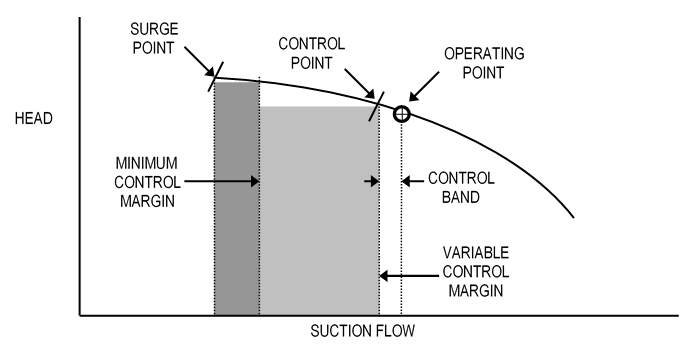
Figure 4: Variable Control Margin Example 1

Figure 5: Variable Control Margin Example 2
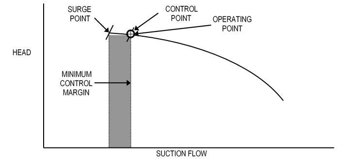
Figure 6: Variable Control Margin Example 3
Variable Margin Equations
The equations for variable control margin are as follows:
Fspt = Ffilt – Fband (6)
where:
Fspt = anti-surge flow controller RSP
Ffilt = anti-surge flow controller MEAS (filtered)
Fband = anti-surge flow control band
The anti-surge flow controller MEAS is filtered (Ffilt) to prevent short-term fluctuations from affecting the variable control margin calculation. The filtering algorithm is implemented as follows:
Ffilt = [Fold * Kfilt] + [Fmeas * (1 – Kfilt)] (7)
where:
Fmeas = anti-surge flow controller MEAS input
Fold = previous value of Ffilt
Kfilt = filter constant (0=no filter)
Anti-Surge Flow Control
The previous sections describe how the setpoint is arrived at for the anti-surge controller. This controller is basically a flow controller that adjusts the anti-surge valve at a frequency of at least 500 ms, and in some applications 100 ms, to control the flow measurement at or above the setpoint. The controller includes several advanced control techniques, which are discussed next.
Adaptive Controller Tuning
The anti-surge flow controller tuning is automatically adjusted depending upon whether the flow is above or below the setpoint. Normal tuning is used when the flow is above setpoint. When the flow is below setpoint, the controller tuning is set faster to quickly return the flow to setpoint. How fast the tuning is set depends upon how far below setpoint the flow has fallen.
Adaptive Tuning Equations
The equations for adaptive tuning are as follows:
Padapt = Pnorm / Kadapt (8)
Iadapt = Inorm / Kadapt (9)
Kadapt = 2 ** {100 * [1 – (Fmeas / Fspt)] / Kdev} (10)
where:
Padapt = adapted PBAND used in anti-surge controller
Pnorm = PBAND setting for normal operation (above control point)
Iadapt = adapted INT used in anti-surge flow controller
Inorm = INT setting for normal operation (above control point)
Kadapt = adaptive tuning factor (limited to a maximum of 1.0)
Fmeas = anti-surge controller MEAS
Fspt = anti-surge controller SPT
Kdev = anti-surge controller negative deviation at which tuning constants are halved (% of SPT)
Asymmetrical Control Action
The adaptive tuning technique previously discussed can result in extremely rapid opening and closing of the anti-surge control valve. This is especially likely as the flow approaches surge because the flow input will become noisier.
To prevent this potential control instability, the SAS compressor controls include asymmetrical control action. This feature allows the anti-surge control valve to open quickly to avoid surge, but close gradually to prevent upsetting other control functions.
Controller Decoupling
The performance controller can sometimes interact with the anti-surge flow controller. This occurs because the performance control action can affect the anti-surge flow as much as the anti-surge control valve does. Therefore, when the compressor is near the surge control point, performance control action can be immediately offset by adjustments to the anti-surge valve. This feature is called controller decoupling.
Surge Line Violation
As the compressor operation approaches the surge line, the flow through the compressor can become erratic. If the flow actually reaches the surge line, then the control margin is automatically increased to push the control line further away from the surge line. An alarm can also be issued, if desired. The margin can increase only up to the maximum margin specified by the engineer.
The control margin can be set back to the original minimum control margin either automatically or manually. The automatic reset is based on elapsed time since the last event. The reset time is set by the engineer. The manual reset is via a button on the anti-surge control graphic display.
Frequent surge line violations are a sign that the minimum control margin is too close to the actual surge point. Therefore, the minimum control margin should be gradually increased until the violations become less frequent.
Performance Control
Performance Control Attributes
The purpose of performance control is to match the throughput of the compressor with the demand for compression. Typical manipulated variables for adjusting throughput are:
- Suction or discharge control valve.
- Inlet guide vanes (IGV).
- Turbine speed for turbine-driven compressors.
- Variable-frequency drive (VFD) for motor-driven compressors.
The demand for compression can be measured by any of the following inputs:
- Suction or discharge pressure.
- Net flow delivered.
Performance control often includes overrides to prevent the violation of other variables, such as:
- Maximum motor amps for motor-driven compressors.
- Minimum suction pressure (when the performance controller is discharge pressure).
- Maximum discharge pressure (when the performance controller is suction pressure).
Air Blower Example
Air blowers are often controlled by a discharge pressure controller that manipulates a suction valve or IGV. A high motor amps override is typically included.
Figure 8 shows an example of the control scheme. The discharge pressure controller (PC) output goes to a split-range (S/R) controller that sends an output to the IGV and the blowoff vent valve according to Table 1. The high amps override is accomplished by a low signal selector (<) that overrides the output to the IGV. If the anti-surge controller (FC) requires more flow, it overrides the S/R output to the blowoff valve via a high signal selector (>).
If the blower has a suction valve instead of an IGV, the controls are exactly the same. If the blower has neither, the S/R, the low selector, and the IGV must be deleted from the scheme in Figure 8. The PC output then goes directly to the high selector.

Figure 8: Performance Control for a Typical Air Blower

Table 1: Discharge Pressure Control Split-Range
Compressor Start-up / Shutdown Ramping
The SAS compressor controls include the ability to ramp the performance controller output upon compressor startup and/or shutdown. The following scenarios are typical and can be adjusted to customer specifications:
- Compressor motor start.
- Compressor loading.
- Compressor unloading.
- Compressor shutdown.
Compressor Motor Start
The operator starts the motor and the compressor comes up to speed in the unloaded position. After detecting the motor start/run via a contact input, the SAS compressor control logic can delay for a preset time period and then ramp the performance control output from the shutdown position to a preset minimum position. The control engineer can specify the delay time, the ramp rate, and the minimum position.
Compressor Loading
After the compressor is started-up in the unloaded position, the operator can initiate compressor loading via a manual entry, or the controls can be configured to automatically load the compressor after motor start. The controls put all necessary controllers in auto, and automatically ramp up the performance valve or compressor speed. The control engineer can specify the ramp rate.
The valve or speed is ramped up until the performance controller, or one of its override controllers, takes over. At any time, the operator can manually suspend the ramp, and manually resume it.
Compressor Unloading
The operator can manually unload the compressor, or the control logic can initiate the unload action. The controls automatically ramp the performance valve or compressor speed to the minimum position. The control engineer can specify the ramp rate.
Compressor Shutdown
When the compressor is shut down, the SAS compressor controls automatically ramp the performance control valve to the shutdown position. The control engineer can specify the ramp rate.
Load Balance
Load Balance Features
In applications involving multiple parallel compressors, a master performance controller is employed to measure the total demand for compression and adjust all compressor performance valves to meet the demand. A typical control scheme is shown in Figure 9, in which a turbine-driven blower and a motor-driven blower are operating in parallel.
In this case, the process demand is indicated by the discharge header pressure. Therefore, performance control consists of a single header pressure controller (PC) adjusting the turbine governor and the suction valve through two bias controllers (HC). The bias allows one blower to be adjusted up or down versus the other.
The header pressure controller in Figure 9 can control the pressure at any combination of governor and suction valve positions. For example, blower A governor could be near minimum speed while blower B suction valve is near wide open. The objective of Load Balance is to adjust the governor and suction valve positions to balance the loads on the blowers. This is done by manipulating the bias controllers shown in Figure 9.

Figure 9: Typical Load Balance Control Scheme
Percent Surge Calculation
Compressor load is measured by calculating the relative distance of the current operating point from the surge control point. This value is expressed as “percent surge” and is calculated as follows:
Load = 100 * [(Fmeas / Fmin) – 1] (11)
where:
Load = compressor load (% of surge)
Fmin = minimum control point
Fmeas = anti-surge controller MEAS input
The reason that percent surge is used for load balance is to prevent one compressor from recycling before the other. Recycle greatly reduces a compressor’s efficiency, and should be used only to prevent surge.
Percent Surge Calculation – Both Recycle Valves Open
Equation 11 works well for compressors that are operating above the surge control point. However, when both compressors are controlling at the control point, both loads are zero, even though their loads may be completely different. Therefore, a way is needed to determine the relative loads under this condition. This is done by modifying equation 11 to include the discharge pressure difference, as follows:
Load = 100 * [(Fmeas / Fmin) – 1] – [Kdp * (PDdisch] (12)
where:
Kdp = Discharge pressure deviation scaling factor
PDdisch = Discharge pressure difference between this compressor and the other compressor (psi)
Equation 12 allows the load calculation to go negative when the anti-surge controllers are controlling at the minimum control point. Therefore, Load Balance can bring the compressors out of recycle simultaneously, as well as into recycle simultaneously.
Percent Surge Calculation – Filtering
The calculated load is filtered to prevent short-term fluctuations from affecting the control action. The filtering algorithm is implemented as follows:
Lfilt = [Lold * Kfilt] + [Lcalc * (1 – Kfilt)] (13)
where:
Lfilt = filtered load
Lcalc = calculated load
Lold = previous value of Lfilt
Kfilt = filter constant (0=no filter)
Percent Surge Examples
Assume that two compressors in parallel are each operating with an anti-surge control point at 400 MSCFH and current flow at 600 MSCFH. The percent surge would be 50% for each compressor because the flow is 200 MSCFH above the surge control point, which is 50% of 400 MSCFH. The two loads would be in balance.
Now assume that the compressors in the previous example are operating at their control points. Therefore, both percent surge values would be zero without considering the discharge pressure difference. However, assume that compressor A discharge pressure is 10 psig while compressor B discharge pressure is 11 psig. If the scaling factor is 10.0, then the percent surge for the first compressor would be -10% while the second would be +10%. In this case, the modified percent surge values indicate that the first compressor is less loaded than the second, which is the actual situation.
Load Balance Control Action
The Load Balance Controller executes at the frequency specified by the control engineer (typically once per minute). Each execution, it obtains the percent surge values for each compressor to be manipulated and calculates the average percent surge. The average is used as the target for each compressor. The controller then adjusts the bias controller bias values to bring each compressor to the average percent surge.
The control equation for each compressor is as follows:
Bdel = Kbal * (Loadavg – Load) (14)
where:
Bdel = change in bias controller BIAS
Kbal = load balance gain factor
Load = compressor load (% of surge)
Loadavg = average compressor load (% of surge)
The Load Balance Controller limits each bias change to a maximum before applying the change to the bias controller. If the load error (Loadavg – Load) is within the engineer-entered deadband, then the error is considered to be zero and no bias change is made.
Excluding Compressor from Load Balance
A compressor will be excluded from load balance when any one of the following conditions occurs:
- compressor is not running.
- compressor is not loaded.
- bias controller is in manual.
- anti-surge flow input is bad.
A compressor may also be excluded when its speed or suction valve position is at maximum. This will happen only when the Load Balance Controller determines that it must increase the bias. If it determines that the bias must be decreased, then the compressor is not excluded.
Similar rules apply to compressors whose speed or suction valve position is at minimum. The compressor is excluded if the controller needs to decrease the bias. It is not excluded when the bias must be increased.
Load Balance Control Example 1
Assume that two compressors are operating as shown in Table 2. Compressor A is operating further away from its surge point than B. Therefore, compressor A load must be reduced by decreasing its bias and B must be loaded up some to offset the decrease in A.

Table 2: Load Balance Example 1
Load Balance Control Example 2
Assume that two compressors are operating as shown in Table 3. Both compressors are operating at their control points, but compressor A discharge pressure is lower than B. The calculated percent surge indicates that A is less loaded than B since A’s discharge pressure is lower than B’s. Therefore, blower A load must be increased by increasing its bias and B must be decreased some to offset the increase in A.

Table 3: Load Balance Example 2
Load Balance Control – Minimum Progress
The load balance control action described above is basically integral-only control operating at an engineer-specified frequency. If the frequency is set faster than the settling time, the percent surge values could oscillate. Therefore, logic has been included to suspend control action whenever the percent surge values are making minimum progress toward the target.
Compressor Sequencing
The SAS compressor controls can also sequence the loading and unloading of parallel compressors based on the current demand for compression. As demand increases, an additional compressor can be loaded based upon a priority list. As demand decreases, the compressor with the highest priority can be unloaded. Optionally, compressors can be automatically started prior to being loaded and stopped after being unloaded. The operator can designate which compressors can participate and set the priority for each compressor.
The application keeps track of compressor start frequency and will bypass a high priority compressor if it is at the maximum number of starts. In addition, the application waits for a compressor to come fully into service before evaluating whether it needs another compressor.
Input Checking
The SAS compressor control logic checks each input and takes appropriate action in the event of a bad value. The following inputs are checked:
- Anti-surge flow input
When a bad input is detected, the anti-surge controller input is set slightly above zero thus causing the anti-surge valve to go wide open.
- Pressures and Temperatures
The suction pressure, suction temperature, discharge pressure and discharge temperature are limited to minimum and maximum values. When a bad input is detected, these inputs are set to the safest possible setpoint for the anti-surge controller.
Foxboro I/A Implementation
The SAS compressor controls are implemented via standard Foxboro I/A blocks. Each compressor has its own compound containing a similar set of blocks. Within each compound, the anti-surge control blocks appear first, followed by the performance control blocks. The load balance blocks are in a separate compound.
A single CP40 can host up to five compressor control packages operating at 100 ms execution frequency. An FCP270 can host even more packages, but multiple compressors are typically distributed among several control processors. Therefore, the number of compressors in a single CP is seldom more than two.
A plot of pressure ratio versus flow is included for each blower. It can be called up from the process display by clicking the mouse on a button labeled XY PLOT. For dual parallel compressors, both blower plots can be configured to appear side-by-side, as shown in Figure 10.
The surge line appears in red and the minimum control line appears in blue. The current operating point is shown as a black square. The operating point is continuously updated to reflect the current conditions. Previous positions of the operating point appear as light green squares.
