Introduction
Advanced Level Control (ALC) is an Advanced Regulatory Control algorithm that provides improved level control action compared to a standard PID controller. ALC minimizes changes in the manipulated flow rate while maintaining the level within the desired operating zone. In addition, feedforward action can be applied to the manipulated flow where appropriate.
Unlike most advanced level control techniques, ALC does not employ non-linear gain. Non-linear gain increases the proportional control action as the level deviates from setpoint. This works fine when the level is moving away from setpoint. However, when the level turns and starts heading back, the proportional action drives the flow in the opposite direction, thus aggressively resisting the return to setpoint.
The better approach, which happens to be the ALC approach, is to take more aggressive control action only when the level is outside of the desired operating zone and moving away from the zone. After the level turns, the control action should be minimal, thus allowing the level to line out as it returns to the desired operating zone.
Standard Level Control Example
Advanced Level Control improves the performance of a standard level controller. An example of a standard level controller is shown in Figure 1. In the example, a feed stream on flow control (FC) is sent to a distillation tower. The tower separates the feed into an overhead stream and a bottoms stream. The bottoms stream, also on flow control (FC), becomes the feed to another tower downstream. The tower bottom level signal (LT) is sent to a level controller (LC) that adjusts the setpoint of the bottoms flow controller in a cascade arrangement.
Note: The drawings in this document use a box containing the letters “FC” to represent a flow controller. When a box is sitting on a process line, then the box also represents the flow transmitter and flow control valve associated with the flow controller.

Figure 1: Standard Level Controller Example
Standard Level Control Proportional Action
The standard level controller uses proportional and integral (PI) action to adjust the bottoms flow to keep the level at setpoint. Proportional (P) action adjusts the flow in proportion to changes in the level. Figure 2 shows an example of proportional action. Notice that when the level goes up, the level controller increases the flow. Likewise, when the level goes down, the level controller decreases the flow. When the level does not change, the flow does not change.
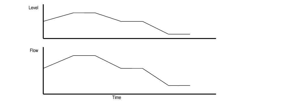
Figure 2: Proportional Control Action Example
Standard Level Control Integral Action
Integral (I) action adjusts the flow in proportion to the error, which is the difference between the current level and the level setpoint. Figure 3 shows an example of integral action. Notice that when the level is above setpoint, the level controller continuously increases the flow setpoint. The rate of increase depends upon how far away the level is from the setpoint. When the level returns to setpoint, the flow is not changed until the level moves away.
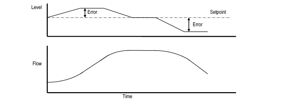
Figure 3: Integral Control Action Example
Standard Level Control Deficiencies
As the examples show, the standard level controller will move the flow around unless the level is right at setpoint and not moving. However, having the level right at setpoint is not really very important; anywhere nearby will usually do fine. In fact, minimizing the changes to the bottoms flow is far more important because the downstream tower will benefit greatly from a steadier flow.
Another problem with the standard level controller is that it cannot offset disturbances that are coming at it until it is too late. Figure 4 shows an example of a feed rate disturbance. The feed flow is suddenly decreased, which will require a decrease in the bottoms flow to prevent losing the bottom level. However, the level controller cannot react until the level itself starts falling sometime after the feed rate change. Then, the level controller must quickly decrease the bottoms flow to prevent losing the level. The level may overshoot on the way back up, causing a roller-coaster effect on the bottoms flow.
In summation, standard level controllers have the following problems:
- They constantly move the flow around unless the level is exactly at setpoint and not moving.
- They react too late to a feed rate disturbance, thus having to move the bottoms flow drastically to catch the level.
In the next section, we will see how Advanced Level Control deals with these control problems.
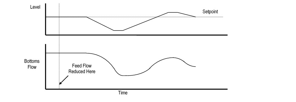
Figure 4: Feed Rate Disturbance Example
Advanced Level Control Features
Advanced Level Control (ALC) is an advanced regulatory control algorithm that is connected to an existing level controller. The algorithm logic is designed to improve level control action by imposing the following rules:
- Take proportional control action only when the level changes by a significant amount.
- Take integral control action only when the level is outside of the desirable operating zone and getting worse.
- Take feedforward control action to lessen the impact of a measurable disturbance on the level.
Let’s look at each of these rules individually using the level control example discussed previously. Figure 5 shows the ALC logic added to the example originally shown in Figure 1. ALC picks up the level signal (LT) and the feed rate (FC) and adjusts various parameters in the level controller (LC).
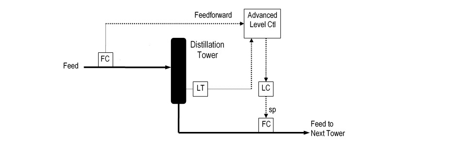
Figure 5: Advanced Level Control Example
Rule #1: Proportional Control Action
Level signals are often quite noisy. They can be filtered somewhat to reduce high-frequency (quick, jumpy) noise, but low-frequency (gradual, rolling) noise is difficult to remove.
ALC minimizes the noise problem by ignoring any changes in the level that do not exceed a significant change limit. Therefore, no proportional control action is taken as long as the level stays inside the significant change limits. Each time the limits are violated, proportional control action is taken and the limits are reset according to the new level. Figure 6 shows how this is done.
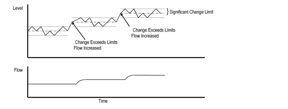
Figure 6: ALC Proportional Control Action Example
Rule #2: Integral Control Action
Integral control action should be suppressed if the level is inside of the desirable operating zone around the setpoint. Even if the level is outside of the zone but heading back, integral action should still be suppressed. Figure 7 illustrates this rule.
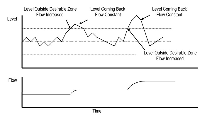
Figure 7: ALC Integral Control Action Example
Rule #3: Feedforward Control Action
Feed rate changes take some time to show up at the bottom level. This time period is referred to as a lag. When the lag time is up and the level starts moving, the standard level controller must quickly adjust the bottoms flow to maintain the level. Figure 4 showed us what usually happens to the bottoms flow in this case.
A better way to adjust the bottoms flow would be:
- watch for a change in the feed rate;
- determine how much the bottoms flow must ultimately be changed to offset the feed rate change;
- gradually ramp the bottoms flow to the new rate during the lag time;
- let the level rise a little at the beginning of the ramp so that the bottoms flow can be smoothly changed over the entire lag time.
ALC automatically performs steps 1 – 4. Figure 8 shows how the level and bottoms flow should respond to a feed flow decrease when ALC is on control.
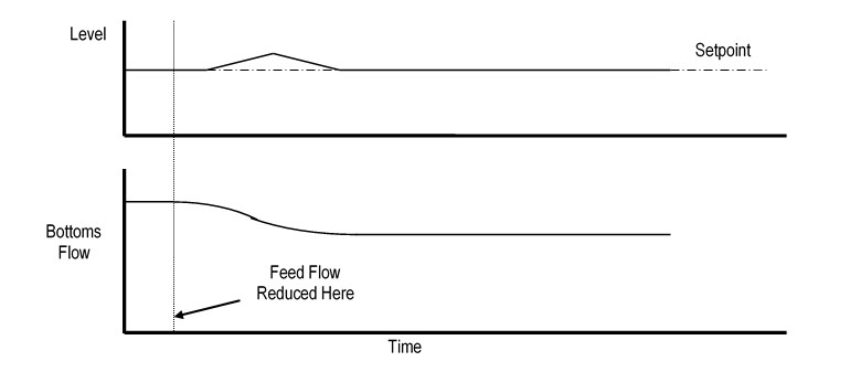
Figure 8: ALC Feedforward Control Action Example
ALC Control Zones
The ALC algorithm operates based on control zones that are evenly spaced around the setpoint. Previously in this document, the term “desirable operating zone” was used to describe the region near the setpoint in which integral control action can be safely suppressed. Outside of that zone, integral action is taken whenever the level is moving away from the zone.
In ALC, the region outside of the desirable operating zone is divided into two zones called the moderate control action zone and the aggressive control action zone. As the names imply, the further away the level is from setpoint, the stronger the control action must be to return the level to the desirable operating zone.
Figure 9 shows the three control zones. The boundary between the desirable and the moderate control action zones is defined by the parameter IBAND1, where IBAND stands for Integral Band. Likewise, the parameter IBAND2 defines the boundary between the moderate control action zone and the aggressive control action zone.
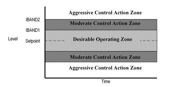
Figure 9: ALC Control Zones
ALC Tuning Parameters
The reason for defining these zones is so that two important tuning parameters, the integral time and the desired minimum progress to setpoint, can be specified separately for each zone. Typically, the integral time is set to 9999 for the desired operating zone, between 10 and 30 minutes for the moderate control action zone, and 5 to 10 minutes for the aggressive control action zone.
The minimum significant progress parameter applies only to the two outermost zones. It specifies how much the level must move toward the setpoint before the integral action is suppressed. In the moderate control action zone, the minimum progress should be set to zero, meaning that the level need only line out or start heading toward setpoint to suppress the integral action. In the aggressive control action zone, the minimum progress should be set above zero to ensure that the ALC drives the level back into the moderate control action zone.
For example, if the minimum progress is 0.1%, the level setpoint is 50.0%, the IBAND2 is 20.0%, and the level decreases from 75.0% to 74.8% in one execution, then the integral action is suppressed. However, if the level stays at 75.0%, then the integral time for the aggressive control action zone is used to drive the level down.
Feedforward Control Action
Feedforward control action is included whenever the manipulated flow needs to be adjusted for changes in another flow that affects the level. This feature is especially useful in feed maximization applications involving several levels in series. When the feed maximization application adjusts the feed rate, the feedforward action simultaneously adjusts the downstream flows to lessen the response time of the process.
It should be noted that feedforward control action is somewhat inconsistent with the objective of ALC, which is minimizing manipulated flow changes. Feedforward actually causes the manipulated flow to move more often than the ALC algorithm would normally allow. Therefore, feedforward should be included only when it is desirable to reduce process response time, or when feedforward flow changes are so large compared to the vessel capacity that the level may go out of control without it.
Feedforward control action is implemented as follows:
- apply dynamic compensation to the feedforward input (if needed);
- calculate the input change from the previous execution;
- multiply the change by a gain factor (note: the gain can include an adaptive factor, if desired);
- add the result to the manipulated flow setpoint via the advanced level controller output.
Feedforward Dynamic Compensation
In general, dynamic compensation is performed by a lead-lag function. The lead element provides an initial boost to the feedforward input, and the lag element provides a first-order lagged response to a step change in the input.
In an ALC application, lead is not desired because it results in excessive changes to the manipulated flow rate. Lag, being much more gradual, is better suited to ALC. The lag is adjusted to the dynamics of the actual level application via the first-order lag time constant, which is the time required for the lag output to reach 63% of the ultimate response to a step change in the input.
Incremental Feedforward Calculation
The change in the feedforward input must be converted to an equivalent change in the manipulated flow. The conversion factor is the adaptive gain. The calculation is as follows:
DelFmanip = Kff * (Fcurr – Fprev) (1)
where:
DelFmanip = Change in manipulated flow rate
Kff = Feedforward gain
Fcurr = Current feedforward lagged input
Fprev = Previous feedforward lagged input
Feedforward Gain
The feedforward gain Kff in equation 1 actually consists of two factors, adaptive gain and attenuation gain:
Kff = K * Kadapt (2)
where:
K = Attenuation gain
Kadapt = Adaptive feedforward gain
The attenuation gain K is used to reduce the calculated feedforward action to attenuate the response. It is usually set between 0.2 (large attenuation) and 1.0 (no attenuation). The adaptive gain converts the change in the feedforward input into an equivalent change in the manipulated flow. It is discussed in more detail below.
Feedforward Adaptive Gain
In the special case of level control applications, the adaptive gain can be calculated as the ratio of the manipulated flow to the feedforward flow as follows:
Kadapt = Fmanip / Ffdfwd (3)
where:
Kadapt = Adaptive feedforward gain
Fmanip = Manipulated flow
Ffdfwd = Feedforward input
By continuously calculating this ratio, the gain is adapted to the current operating conditions. To prevent noise or other short-term flow fluctuations from adversely affecting the feedforward action, the calculated adaptive gain is averaged, as follows:
Kavg = [Knew * (1 – Clag)] + [Kold * Clag] (4)
where:
Knew = Newly calculated adaptive feedforward gain
Kold = Previous value of Kavg
Clag = Lag constant (0.0 to 1.0 where 0.0=no lag)
The lag constant Clag is defined as follows:
Clag = EXP [ts / (60 * tau)] (5)
where:
ts = Block execution interval (sec)
tau = First-order lag time constant (min)